import numpy as np
import matplotlib.pyplot as plt
from scipy.optimize import minimize_scalar
np.random.seed(214)
# Define the quadratic function and its gradient
def quadratic_function(x, A, b):
return 0.5 * np.dot(x.T, np.dot(A, x)) - np.dot(b.T, x)
def grad_quadratic(x, A, b):
return np.dot(A, x) - b
# Generate a 2D quadratic problem with a specified condition number
def generate_quadratic_problem(cond_number):
# Random symmetric matrix
M = np.random.randn(2, 2)
M = np.dot(M, M.T)
# Ensure the matrix has the desired condition number
U, s, V = np.linalg.svd(M)
s = np.linspace(cond_number, 1, len(s)) # Spread the singular values
A = np.dot(U, np.dot(np.diag(s), V))
# Random b
b = np.random.randn(2)
return A, b
# Gradient descent function
def gradient_descent(start_point, A, b, stepsize_func, max_iter=100):
x = start_point.copy()
trajectory = [x.copy()]
for i in range(max_iter):
grad = grad_quadratic(x, A, b)
step_size = stepsize_func(x, grad)
x -= step_size * grad
trajectory.append(x.copy())
return np.array(trajectory)
# Backtracking line search strategy using scipy
def backtracking_line_search(x, grad, A, b, alpha=0.3, beta=0.8):
def objective(t):
return quadratic_function(x - t * grad, A, b)
res = minimize_scalar(objective, method='golden')
return res.x
# Generate ill-posed problem
cond_number = 30
A, b = generate_quadratic_problem(cond_number)
# Starting point
start_point = np.array([1.0, 1.8])
# Perform gradient descent with both strategies
trajectory_fixed = gradient_descent(start_point, A, b, lambda x, g: 5e-2)
trajectory_backtracking = gradient_descent(start_point, A, b, lambda x, g: backtracking_line_search(x, g, A, b))
# Plot the trajectories on a contour plot
x1, x2 = np.meshgrid(np.linspace(-2, 2, 400), np.linspace(-2, 2, 400))
Z = np.array([quadratic_function(np.array([x, y]), A, b) for x, y in zip(x1.flatten(), x2.flatten())]).reshape(x1.shape)
plt.figure(figsize=(10, 8))
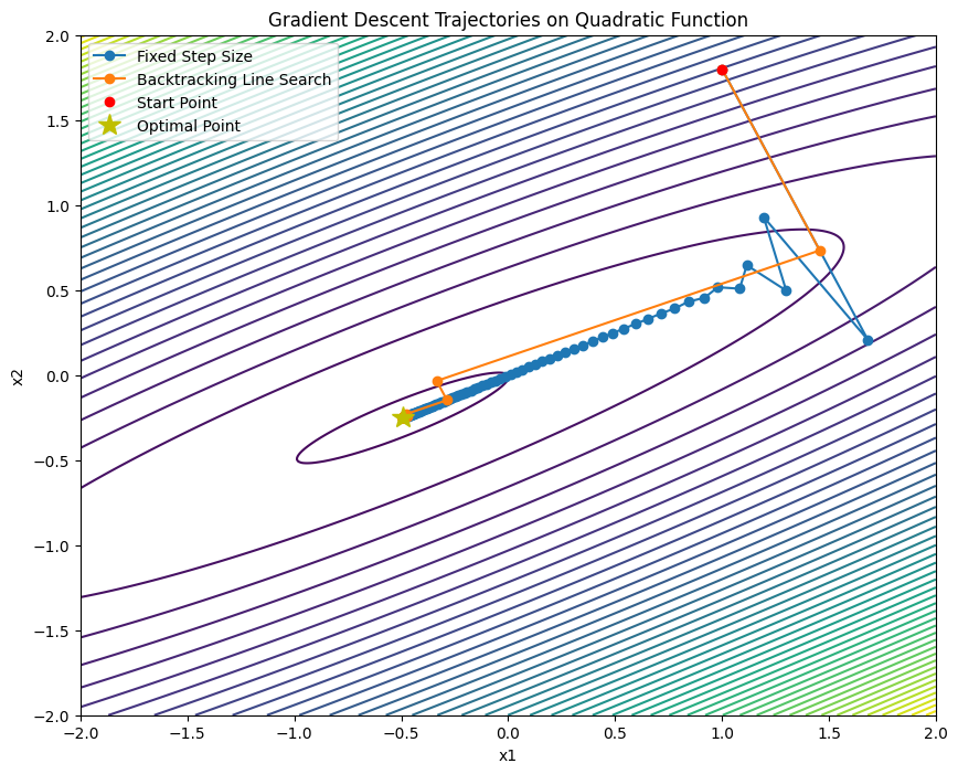
plt.contour(x1, x2, Z, levels=50, cmap='viridis')
plt.plot(trajectory_fixed[:, 0], trajectory_fixed[:, 1], 'o-', label='Fixed Step Size')
plt.plot(trajectory_backtracking[:, 0], trajectory_backtracking[:, 1], 'o-', label='Backtracking Line Search')
# Add markers for start and optimal points
plt.plot(start_point[0], start_point[1], 'ro', label='Start Point')
optimal_point = np.linalg.solve(A, b)
plt.plot(optimal_point[0], optimal_point[1], 'y*', markersize=15, label='Optimal Point')
plt.legend()
plt.title('Gradient Descent Trajectories on Quadratic Function')
plt.xlabel('x1')
plt.ylabel('x2')
plt.savefig("linesearch.svg")
plt.show()